Much of the information here was taken from Ian Frost's description of his Chaotic Pendulum java app.
Dynamical systems are often modelled by a set of n first order differential equations:
dx/dt = F(x(t)) ............... (*)
where x is a vector in phase space and F is a vector field over this space. The coordinates of phase space are the variables which are necessary to completely describe the instantaneous state of a dynamical system ie each component of x. For chaotic behaviour to be possible there needs to be some nonlinearity and the dimension, n, of phase space must be at least 3. One of the simplest dynamical systems which satisfies these conditions is the forced pendulum.
A damped, sinusoidally driven pendulum of mass m (or weight W) and length l is described by the following equation of motion:
mld2![]() /dt2 +
/dt2 + ![]() d
d![]() /dt + Wsin
/dt + Wsin![]() = Acos(
= Acos(![]() Dt)
Dt)
where the left hand terms represent acceleration, damping and gravitation, and the right hand side is the forcing term. In dimensionless form the equation can be rewritten as:
d2![]() /dt2
+ (1/q)d
/dt2
+ (1/q)d![]() /dt
+ sin
/dt
+ sin![]() = gcos(
= gcos(![]() Dt)
Dt)
where q is the damping factor, g is the forcing
amplitude and ![]() D
is the angular forcing frequency. In the form of equation (*) we
have:
D
is the angular forcing frequency. In the form of equation (*) we
have:
d![]() /dt
= -(1/q)
/dt
= -(1/q)![]() - sin
- sin![]() + gcos
+ gcos![]()
d![]() /dt
=
/dt
= ![]()
d![]() /dt =
/dt = ![]() D
D
where ![]() is
the angular frequency,
is
the angular frequency, ![]() is the angular position, and
is the angular position, and ![]() is the phase of the
forcing term. (
is the phase of the
forcing term. (![]() ,
,![]() ,
,![]() ) are the three
dynamic variables necessary for chaos and the sin
) are the three
dynamic variables necessary for chaos and the sin![]() and cos
and cos![]() terms provide the
nonlinearity. The pendulum displays a variety of ordered and
chaotic behaviour depending on the values of the parameters g,
terms provide the
nonlinearity. The pendulum displays a variety of ordered and
chaotic behaviour depending on the values of the parameters g,![]() D and q.
D and q.
For small oscillations the undamped pendulum has a natural angular frequency of unity in the units employed here. Chaotic behaviour arises partly from the interaction between the driving frequency and the natural frequency so we can expect to find interesting behaviour for driving frequencies close to 1.
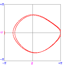
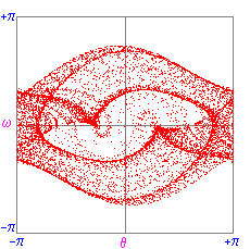
The pendulum has a 3-dimensional phase space with ![]() ,
,![]() ,
,![]() as the coordinate
axes. The phase trajectory is projected onto the (
as the coordinate
axes. The phase trajectory is projected onto the (![]() ,
,![]() ) plane. In this
plane periodic motion appears as closed loops.
) plane. In this
plane periodic motion appears as closed loops.
 |
 |
| Periodic state: g=1.07, q=2,
|
Chaotic state: g=1.15, q=2,
|
As a transition to chaos occurs the picture becomes more
complicated and can be simplified by the use of the Poincare
section. The section is constructed by sampling the phase space
diagram stroboscopically. In this case the strobe period is the
period of the forcing. In this way, a cross-section of the
3-dimensional attractor is taken at a position along the ![]() axis. Periodic orbits
are now represented as a finite set of points, while chaotic
orbits comprise infinitely many points.
axis. Periodic orbits
are now represented as a finite set of points, while chaotic
orbits comprise infinitely many points.
 |
 |
| Periodic state: g=1.07, q=2,
|
Chaotic state: g=1.15, q=2,
|