• General Purpose
• Power Analysis and Sample Size Calculation in Experimental Design
  • Sampling Theory
  • Hypothesis Testing Logic
  • Calculating Power
  • Calculating Required Sample Size
  • Graphical Approaches to Power Analysis
• Noncentrality Interval Estimation and the Evaluation of Statistical Models
  • Inadequacies of the Hypothesis Testing Approach
  • Advantages of Interval Estimation
  • Reasons Why Interval Estimates are Seldom Reported
  • Replacing Traditional Hypothesis Tests with Interval Estimates

The techniques of statistical power analysis, sample size estimation, and advanced techniques for confidence interval estimation are discussed here. The main goal of first the two techniques is to allow you to decide, while in the process of designing an experiment, (a) how large a sample is needed to enable statistical judgments that are accurate and reliable and (b) how likely your statistical test will be to detect effects of a given size in a particular situation. The third technique is useful in implementing objectives a and b and in evaluating the size of experimental effects in practice.

Performing power analysis and sample size estimation is an important aspect of experimental design, because without these calculations, sample size may be too high or too low. If sample size is too low, the experiment will lack the precision to provide reliable answers to the questions it is investigating. If sample size is too large, time and resources will be wasted, often for minimal gain.

In some power analysis software programs, a number of graphical and analytical tools are available to enable precise evaluation of the factors affecting power and sample size in many of the most commonly encountered statistical analyses. This information can be crucial to the design of a study that is cost-effective and scientifically useful.

Noncentrality interval estimation procedures and other sophisticated confidence interval procedures provide some sophisticated confidence interval methods for analyzing the importance of an observed experimental result. An increasing number of influential statisticians are suggesting that confidence interval estimation should augment or replace traditional hypothesis testing approaches in the analysis of experimental data.

To index

Power Analysis and Sample Size Calculation in Experimental Design

There is a growing recognition of the importance of power analysis and sample size calculation in the proper design of experiments. Click on the links below for a discussion of the fundamental ideas behind these methods.

• Sampling Theory
• Hypothesis Testing Logic
• Calculating Power
• Calculating Required Sample Size
• Graphical Approaches to Power Analysis

Typically, we take a sample and compute a quantity called a statistic in order to estimate some characteristic of a population called a parameter.

For example, suppose a politician is interested in the proportion of people who currently favor her position on a particular issue. Her constituency is a large city with a population of about 1,500,000 potential voters. In this case, the parameter of interest, which we might call , is the proportion of people in the entire population who favor the politician's position. The politician is going to commission an opinion poll, in which a (hopefully) random sample of people will be asked whether or not they favor her position. The number (call it N) of people to be polled will be quite small, relative to the size of the population. Once these people have been polled, the proportion of them favoring the politician's position will be computed. This proportion, which is a statistic, can be called p.

One thing is virtually certain before the study is ever performed: p will not be equal to ! Because p involves "the luck of the draw," it will deviate from . The amount by which p is wrong, i.e., the amount by which it deviates from , is called sampling error.

In any one sample, it is virtually certain there will be some sampling error (except in some highly unusual circumstances), and that we will never be certain exactly how large this error is. If we knew the amount of the sampling error, this would imply that we also knew the exact value of the parameter, in which case we would not need to be doing the opinion poll in the first place.

In general, the larger the sample size N, the smaller sampling error tends to be. (One can never be sure what will happen in a particular experiment, of course.) If we are to make accurate decisions about a parameter like , we need to have an N large enough so that sampling error will tend to be "reasonably small." If N is too small, there is not much point in gathering the data, because the results will tend to be too imprecise to be of much use.

On the other hand, there is also a point of diminishing returns beyond which increasing N provides little benefit. Once N is "large enough" to produce a reasonable level of accuracy, making it larger simply wastes time and money.

So some key decisions in planning any experiment are, "How precise will my parameter estimates tend to be if I select a particular sample size?" and "How big a sample do I need to attain a desirable level of precision?"

The purpose of Power Analysis and Sample Size Estimation is to provide you with the statistical methods to answer these questions quickly, easily, and accurately. A good statistical software program will provide simple dialogs for performing power calculations and sample size estimation for many of the classic statistical procedures as well as special noncentral distribution routines to allow the advanced user to perform a variety of additional calculations.

Hypothesis Testing. Suppose that the politician was interested in showing that more than the majority of people supported her position. Her question, in statistical terms: "Is > .50?" Being an optimist, she believes that it is.

In statistics, the following strategy is quite common. State as a "statistical null hypothesis" something that is the logical opposite of what you believe. Call this hypothesis H0. Gather data. Then, using statistical theory, show from the data that it is likely H0 is false, and should be rejected.

By rejecting H0, you support what you actually believe. This kind of situation, which is typical in many fields of research, for example, is called "Reject-Support testing," (RS testing) because rejecting the null hypothesis supports the experimenter's theory.

The null hypothesis is either true or false, and the statistical decision process is set up so that there are no "ties." The null hypothesis is either rejected or not rejected. Consequently, before undertaking the experiment, we can be certain that only 4 possible things can happen. These are summarized in the table below

		State of the World
		HO	H1
Decision	H0	Correct Acceptance	Type II Error
	H1	Type I Error	Correct Rejection

Note that there are two kinds of errors represented in the table. Many statistics textbooks present a point of view that is common in the social sciences, i.e., that , the Type I error rate, must be kept at or below .05, and that, if at all possible, , the Type II error rate, must be kept low as well. "Statistical power," which is equal to 1 - , must be kept correspondingly high. Ideally, power should be at least .80 to detect a reasonable departure from the null hypothesis.

The conventions are, of course, much more rigid with respect to than with respect to . For example, in the social sciences seldom, if ever, is allowed to stray above the magical .05 mark.

Significance Testing (RS/AS). In the context of significance testing, we can define two basic kinds of situations, reject-support (RS) (discussed above) and accept-support (AS). In RS testing, the null hypothesis is the opposite of what the researcher actually believes, and rejecting it supports the researcher's theory. In a two group RS experiment involving comparison of the means of an experimental and control group, the experimenter believes the treatment has an effect, and seeks to confirm it through a significance test that rejects the null hypothesis.

In the RS situation, a Type I error represents, in a sense, a "false positive" for the researcher's theory. From society's standpoint, such false positives are particularly undesirable. They result in much wasted effort, especially when the false positive is interesting from a theoretical or political standpoint (or both), and as a result stimulates a substantial amount of research. Such follow-up research will usually not replicate the (incorrect) original work, and much confusion and frustration will result.

In RS testing, a Type II error is a tragedy from the researcher's standpoint, because a theory that is true is, by mistake, not confirmed. So, for example, if a drug designed to improve a medical condition is found (incorrectly) not to produce an improvement relative to a control group, a worthwhile therapy will be lost, at least temporarily, and an experimenter's worthwhile idea will be discounted.

As a consequence, in RS testing, society, in the person of journal editors and reviewers, insists on keeping low. The statistically well-informed researcher makes it a top priority to keep low as well. Ultimately, of course, everyone benefits if both error probabilities are kept low, but unfortunately there is often, in practice, a trade-off between the two types of error.

The RS situation is by far the more common one, and the conventions relevant to it have come to dominate popular views on statistical testing. As a result, the prevailing views on error rates are that relaxing beyond a certain level is unthinkable, and that it is up to the researcher to make sure statistical power is adequate. One might argue how appropriate these views are in the context of RS testing, but they are not altogether unreasonable.

In AS testing, the common view on error rates we described above is clearly inappropriate. In AS testing, H0 is what the researcher actually believes, so accepting it supports the researcher's theory. In this case, a Type I error is a false negative for the researcher's theory, and a Type II error constitutes a false positive. Consequently, acting in a way that might be construed as highly virtuous in the RS situation, for example, maintaining a very low Type I error rate like .001, is actually "stacking the deck" in favor of the researcher's theory in AS testing.

In both AS and RS situations, it is easy to find examples where significance testing seems strained and unrealistic. Consider first the RS situation. In some such situations, it is simply not possible to have very large samples. An example that comes to mind is social or clinical psychological field research. Researchers in these fields sometimes spend several days interviewing a single subject. A year's research may only yield valid data from 50 subjects. Correlational tests, in particular, have very low power when samples are that small. In such a case, it probably makes sense to relax beyond .05, if it means that reasonable power can be achieved.

On the other hand, it is possible, in an important sense, to have power that is too high. For example, one might be testing the hypothesis that two population means are equal (i.e., Mu1 = Mu2) with sample sizes of a million in each group. In this case, even with trivial differences between groups, the null hypothesis would virtually always be rejected.

The situation becomes even more unnatural in AS testing. Here, if N is too high, the researcher almost inevitably decides against the theory, even when it turns out, in an important sense, to be an excellent approximation to the data. It seems paradoxical indeed that in this context experimental precision seems to work against the researcher.

To summarize:

In Reject-Support research:

1. The researcher wants to reject H0.
2. Society wants to control Type I error.
3. The researcher must be very concerned about Type II error.
4. High sample size works for the researcher.
5. If there is "too much power," trivial effects become "highly significant."

1. The researcher wants to accept H0.
2. "Society" should be worrying about controlling Type II error, although it sometimes gets confused and retains the conventions applicable to RS testing.
3. The researcher must be very careful to control Type I error.
4. High sample size works against the researcher.
5. If there is "too much power," the researcher's theory can be "rejected" by a significance test even though it fits the data almost perfectly.

1. What kind of statistical test is being performed. Some statistical tests are inherently more powerful than others.
2. Sample size. In general, the larger the sample size, the larger the power. However, generally increasing sample size involves tangible costs, both in time, money, and effort. Consequently, it is important to make sample size "large enough," but not wastefully large.
3. The size of experimental effects. If the null hypothesis is wrong by a substantial amount, power will be higher than if it is wrong by a small amount.
4. The level of error in experimental measurements. Measurement error acts like "noise" that can bury the "signal" of real experimental effects. Consequently, anything that enhances the accuracy and consistency of measurement can increase statistical power.

Let's briefly examine the kind of statistical theory that lies at the foundation of the calculations used to estimate power and sample size. Return to the original example of the politician, contemplating how large an opinion poll should be taken to suit her purposes.

Statistical theory, of course, cannot tell us what will happen with any particular opinion poll. However, through the concept of a sampling distribution, it can tell us what will tend to happen in the long run, over many opinion polls of a particular size.

A sampling distribution is the distribution of a statistic over repeated samples. Consider the sample proportion p resulting from an opinion poll of size N, in the situation where the population proportion is exactly .50. Sampling distribution theory tells us that p will have a distribution that can be calculated from the binomial theorem. This distribution, for reasonably large N, and for values of p not too close to 0 or 1, looks very much like a normal distribution with a mean of and a standard deviation (called the "standard error of the proportion") of

s_p = (p(1-p)/N)**1/2

Suppose, for example, the politician takes an opinion poll based on an N of 100. Then the distribution of p, over repeated samples, will look like this if = .5.

The values are centered around .5, but a small percentage of values are greater than .6 or less than .4. This distribution of values reflects the fact that an opinion poll based on a sample of 100 is an imperfect indicator of the population proportion .

If p were a "perfect" estimate of , the standard error of the proportion would be zero, and the sampling distribution would be a spike located at 0.5. The spread of the sampling distribution indicates how much "noise" is mixed in with the "signal" generated by the parameter.

Notice from the equation for the standard error of the proportion that, as N increases, the standard error of the proportion gets smaller. If N becomes large enough, we can be very certain that our estimate p will be a very accurate one.

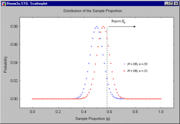
Suppose the politician uses a decision criterion as follows. If the observed value of p is greater than .58, she will decide that the null hypothesis that is less than or equal to .50 is false. This rejection rule is diagrammed below.

One may, by adding up all the probabilities (computable from the binomial distribution), determine that the probability of rejecting the null hypothesis when p = .50 is .044. Hence, this decision rule controls the Type I Error rate, , at or below .044. It turns out, this is the lowest decision criterion that maintains at or below .05.

However, the politician is also concerned about power in this situation, because it is by rejecting the null hypothesis that she is able to support the notion that she has public opinion on her side.

Suppose that 55% of the people support the politician, that is, that = .55 and the null hypothesis is actually false. In this case, the correct decision is to reject the null hypothesis. What is the probability that she will obtain a sample proportion greater than the "cut-off" value of .58 required to reject the null hypothesis?

In the figure below, we have superimposed the sampling distribution for p when = .55. Clearly, only a small percentage of the time will the politician reach the correct decision that she has majority support. The probability of obtaining a p greater than .58 is only .241.

Needless to say, there is no point in conducting an experiment in which, if your position is correct, it will only be verified 24.1% of the time! In this case a statistician would say that the significance test has "inadequate power to detect a departure of 5 percentage points from the null hypothesized value."

The crux of the problem lies in the width of the two distributions in the preceding figure. If the sample size were larger, the standard error of the proportion would be smaller, and there would be little overlap between the distributions. Then it would be possible to find a decision criterion that provides a low and high power.

The question is, "How large an N is necessary to produce a power that is reasonably high" in this situation, while maintaining at a reasonably low value.

One could, of course, go through laborious, repetitive calculations in order to arrive at such a sample size. However, a good software program will perform them automatically, with just a few clicks of the mouse. Moreover, for each analytic situation that it handles, it will provide extensive capabilities for analyzing and graphing the theoretical relationships between power, sample size, and the variables that affect them. Assuming that the user will be employing the well known chi-square test, rather than the exact binomial test, suppose that the politician decides that she requires a power of .80 to detect a p of .80. It turns out, a sample size of 607 will yield a power of exactly .8009. (The actual alpha of this test, which has a nominal level of .05, is .0522 in this situation.)

To index

Graphical Approaches to Power Analysis. In the preceding discussion, we arrived at a necessary sample size of 607 under the assumption that p is precisely .80. In practice, of course, we would be foolish to perform only one power calculation, based on one hypothetical value. For example, suppose the function relating required sample size to p is particularly steep in this case. It might then be that the sample size required for a p of .70 is much different than that required to reliably detect a p of .80.

Intelligent analysis of power and sample size requires the construction, and careful evaluation, of graphs relating power, sample size, the amount by which the null hypothesis is wrong (i.e., the experimental effect), and other factors such as Type I error rate.

In the example discussed in the preceding section, the goal, from the standpoint of the politician, is to plan a study that can decide, with a low probability of error, whether the support level is greater than .50. Graphical analysis can shed a considerable amount of light on the capabilities of a statistical test to provide the desired information under such circumstances.

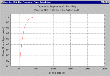
For example, the researcher could plot power against sample size, under the assumption that the true level is .55, i.e., 55%. The user might start with a graph that covers a very wide range of sample sizes, to get a general idea of how the statistical test behaves. The following graph shows power as a function of sample sizes ranging from 20 to 2000, using a "normal approximation" to the exact binomial distribution.

The previous graph demonstrates that power reaches an acceptable level (often considered to be between .80 and .90) at a sample size of approximately 600.

Remember, however, that this calculation is based on the supposition that the true value of p is .55. It may be that the shape of the curve relating power and sample size is very sensitive to this value. The question immediately arises, "how sensitive is the slope of this graph to changes in the actual value of p?

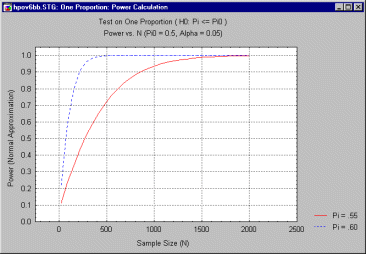
There are a number of ways to address this question. One can plot power vs. sample size for other values of p, for example. Below is a graph of power vs. sample size for p = .6.

One can see immediately in the preceding graph that the improvement in power for increases in N occurs much more rapidly for p = .6 than for p = .55. The difference is striking if you merge the two graphs into one, as shown below.

In planning a study, particularly when a grant proposal must be submitted with a proposed sample size, one must estimate what constitutes a reasonable minimum effect that one wishes to detect, a minimum power to detect that effect, and the sample size that will achieve that desired level of power. This sample size can be obtained by analyzing the above graphs (additionally, some software packages can calculate it directly). For example, if the user requests the minimum sample size required to achieve a power of .90 when p = .55, some programs can calculate this directly. The result is reported in a spreadsheet, as below,

	One Proportion, Z (or Chi-Square) Test H0: Pi < = Pi0
	Value
Null Hypothesized Proportion (Pi0)	.5000
Population Proportion (Pi)	.5500
Alpha (Nominal)	.0500
Required Power	.9000
Required Sample Size (N)	853.0000
Actual Alpha (Exact)	.0501
Power (Normal Approximation)	.9001
Power (Exact)	.9002

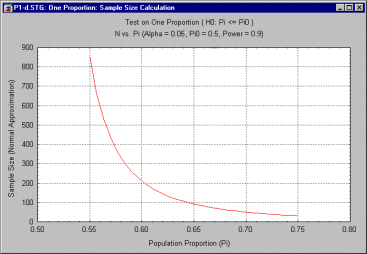
For a given level of power, a graph of sample size vs. p can show how sensitive the required sample size is to the actual value of p. This can be important in gauging how sensitive the estimate of a required sample size is. For example, the following graph shows values of N needed to achieve a power of .90 for various values of p, when the null hypothesis is that p = .50

The preceding graph demonstrates how the required N drops off rapidly as p varies from .55 to .60. To be able to reliably detect a difference of .05 (from the null hypothesized value of .50) requires an N greater than 800, but reliable detection of a difference of .10 requires an N of only around 200. Obviously, then, required sample size is somewhat difficult to pinpoint in this situation. It is much better to be aware of the overall performance of the statistical test against a range of possibilities before beginning an experiment, than to be informed of an unpleasant reality after the fact. For example, imagine that the experimenter had estimated the required sample size on the basis of reliably (with power of .90) detecting a p of .6. The experimenter budgets for a sample size of, say, 220, and imagines that minor departures of p from .6 will not require substantial differences in N. Only later does the experimenter realize that a small change in requires a huge increase in N , and that the planning for the experiment was optimistic. In some such situations, a "window of opportunity" may close before the sample size can be adjusted upward.

Across a wide variety of analytic situations, Power analysis and sample size estimation involve steps that are fundamentally the same.

1. The type of analysis and null hypothesis are specified
2. Power and required sample size for a reasonable range of effects is investigated.
3. The sample size required to detect a reasonable experimental effect (i.e., departure from the null hypothesis), with a reasonable level of power, is calculated, while allowing for a reasonable margin of error.

Power Analysis and Interval Estimation includes a number of confidence intervals that are not widely available in general purpose statistics packages. Several of these are discussed within a common theoretical framework, called "noncentrality interval estimation," by Steiger and Fouladi (1997). In this section, we briefly review some of the basic rationale behind the emerging popularity of confidence intervals.

Inadequacies of the Hypothesis Testing Approach. Strictly speaking, the outcome of a significance test is the dichotomous decision whether or not to reject the null hypothesis. This dichotomy is inherently dissatisfying to many scientists who use the null hypothesis as a statement of no effect, and are more interested in knowing how big an effect is than whether it is (precisely) zero. This has led to behavior like putting one, two, or three asterisks next to results in tables, or listing p levels next to results, when, in fact, such numbers, across (or sometimes even within!) studies need not be monotonically related to the best estimates of strength of experimental effects, and hence can be extremely misleading. Some writers (e.g., Guttman, 1977) view asterisk-placing behavior as inconsistent with the foundations of significance testing logic.

Probability levels can deceive about the "strength" of a result, especially when presented without supporting information. For example, if, in an ANOVA table, one effect had a p level of .019, and the other a p level of .048, it might be an error to conclude that the statistical evidence supported the view that the first effect was stronger than the second. A meaningful interpretation would require additional information. To see why, suppose someone reports a p level of .001. This could be representative of a trivial population effect combined with a huge sample size, or a powerful population effect combined with a moderate sample size, or a huge population effect with a small sample. Similarly a p level of .075 could represent a powerful effect operating with a small sample, or a tiny effect with a huge sample. Clearly then, we need to be careful when comparing p levels.

In Accept-Support testing, which occurs frequently in the context of model fitting in factor analysis or "causal modeling," significance testing logic is basically inappropriate. Rejection of an "almost true" null hypothesis in such situations frequently has been followed by vague statements that the rejection shouldn't be taken too seriously. Failure to reject a null hypothesis usually results in a demand by a vigilant journal editor for cumbersome power calculations. Such problems can be avoided to some extent by using confidence intervals.

To index

Advantages of Interval Estimation. Much research is exploratory. The fundamental questions in exploratory research are "What is our best guess for the size of the population effect?" and "How precisely have we determined the population effect size from our sample data?" Significance testing fails to answer these questions directly. Many a researcher, faced with an "overwhelming rejection" of a null hypothesis, cannot resist the temptation to report that it was "significant well beyond the .001 level." Yet it is widely agreed that a p level following a significance test can be a poor vehicle for conveying what we have learned about the strength of population effects.

Confidence interval estimation provides a convenient alternative to significance testing in most situations. Consider the 2-tailed hypothesis of no difference between means. Recall first that the significance test rejects at the significance level if and only if the 1 - confidence interval for the mean difference excludes the value zero. Thus the significance test can be performed with the confidence interval. Most undergraduate texts in behavioral statistics show how to compute such a confidence interval. The interval is exact under the assumptions of the standard t test. However, the confidence interval contains information about experimental precision that is not available from the result of a significance test. Assuming we are reasonably confident about the metric of the data, it is much more informative to state a confidence interval on Mu1 - Mu2 than it is to give the p level for the t test of the hypothesis that Mu1 - Mu2 = 0 In summary, we might say that, in general, a confidence interval conveys more information, in a more naturally usable form, than a significance test.

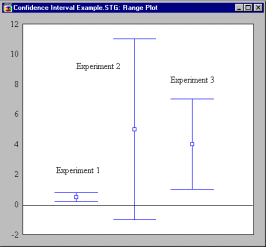
This is seen most clearly when confidence intervals from several studies are graphed alongside one another, as in the figure below

The figure shows confidence intervals for the difference between means for 3 experiments, all performed in the same domain, using measures with approximately the same variability. Experiments 1 and 3 yield a confidence interval that fails to include zero. For these experiments, the null hypothesis was rejected. The second experiment yields a confidence interval that includes zero, so the null hypothesis of no difference is not rejected. A significance testing approach would yield the impression that the second experiment did not agree with the first and the third.

The confidence intervals suggest a different interpretation, however. The first experiment had a very large sample size, and very high precision of measurement, reflected in a very narrow confidence interval. In this experiment, a small effect was found, and determined with such high precision that the null hypothesis of no difference could be rejected at a stringent significance level.

The second experiment clearly lacked precision, and this is reflected in the very wide confidence interval. Evidently, the sample size was too small. It may well be that the actual effect in conditions assessed in the second experiment was larger than that in the first experiment, but the experimental precision was simply inadequate to detect it.

The third experiment found an effect that was statistically significant, and perhaps substantially higher than the first experiment, although this is partly masked by the lower level of precision, reflected in a confidence interval that, though narrower than Experiment 2, is substantially wider than Experiment 1.

Suppose the 3 experiments involved testing groups for differences in IQ. In the final analysis, we may have had too much power in Experiment 1, as we are declaring "highly significant" a rather miniscule effect substantially less than a single IQ point. We had far too little power in Experiment 2. Experiment 3 seems about right.

Many of the arguments we have made on behalf of confidence intervals have been made by others as cogently as we have made them here. Yet, confidence intervals are seldom reported in the literature. Most important, as we demonstrate in the succeeding sections, there are several extremely useful confidence intervals that virtually never are reported. In what follows, we discuss why the intervals are seldom reported.

To index

Reasons Why Interval Estimates are Seldom Reported. In spite of the obvious advantages of interval estimates, they are seldom employed in published articles in many areas of science. On those infrequent occasions when interval estimates are reported, they are often not the optimal ones. There are several reasons for this status quo:

Tradition. Traditional approaches to statistics emphasize significance testing much more than interval estimation.

Pragmatism. In RS situations, interval estimates are sometimes embarrassing. When they are narrow but close to zero, they suggest that a "highly significant" result may be statistically significant but trivial. When they are wide, they betray a lack of experimental precision.

Ignorance. Many people are simply unaware of some of the very valuable interval estimation procedures that are available. For example, many textbooks on multivariate analysis never mention that it is possible to compute a confidence interval on the squared multiple correlation coefficient.

Lack of availability. Some of the most desirable interval estimation procedures are computer intensive, and have not been implemented in major statistical packages. This has made it less likely that anyone will try the procedure.

To index

Replacing Traditional Hypothesis Tests with Interval Estimates. There are a number of confidence interval procedures that can replace and/or augment the traditional hypothesis tests used in classical testing situations. For a review of these techniques, see Steiger & Fouladi (1997).

Analysis of Variance. One area where confidence intervals have seldom been employed is in assessing strength of effects in the Analysis of Variance (ANOVA).

For example, suppose you are reading a paper, which reports that, in a 1-Way ANOVA, with 4 groups, and N = 60 per group, an F statistic was found that is significant at the .05 level ("F = 2.70, p =.0464"). This result is statistically significant, but how meaningful is it in a practical sense? What have we learned about the size of the experimental effects?

Fleischman (1980) discusses a technique for setting a confidence interval on the overall effect size in the Analysis of Variance. This technique allows one to set a confidence interval on the RMSSE, the root-mean-square standardized effect. Standardized effects are reported in standard deviation units, and are hence remain constant when the unit of measurement changes. So, for example, an experimental effect reported in pounds would be different from the same effect reported in kilograms, whereas the standardized effect would be the same in each case. In the case of the data mentioned above, the F statistic that is significant at the .05 level yields a 90% confidence interval for the RMSSE that ranges from .0190 to .3139. The lower limit of this interval stands for a truly mediocre effect, less than 1/50th of a standard deviation. The upper limit of the interval represents effects on the order of 1/3 of a standard deviation, moderate but not overwhelming. It seems, then, that the results from this study need not imply really strong experimental effects, even though the effects are statistically "significant."

Multiple Regression. The squared multiple correlation is reported frequently as an index of the overall strength of a prediction equation. After fitting a regression equation, the most natural questions to ask are, (a) "How effective is the regression equation at predicting the criterion?" and (b) "How precisely has this effectiveness been determined?"

Hence, one very common statistical application that practically cries out for a confidence interval is multiple regression analysis. Publishing an observed squared multiple R together with the result of a hypothesis test that the population squared multiple correlation is zero, conveys little of the available statistical information. A confidence interval on the populations squared multiple correlation is much more informative.

One software package computes exact confidence intervals for the population squared multiple correlation, following the approach of Steiger and Fouladi (1992). As an example, suppose a criterion is predicted from 45 independent observations on 5 variables and the observed squared multiple correlation is .40. In this case a 95% confidence interval for the population squared multiple correlation ranges from .095 to .562! A 95% lower confidence limit is at .129. On the other hand the sample multiple correlation value is significant "beyond the .001 level," because the p level is .0009, and the shrunken estimator is .327. Clearly, it is far more impressive to state that "the squared multiple R value is significant at the .001 level" than it is to state that "we are 95% confident that the population squared multiple correlation is between .095 and .562." But we believe the latter statement conveys the quality and meaning of the statistical result more accurately than the former.

Some writers, like Lee (1972), prefer a lower confidence limit, or "statistical lower bound" on the squared multiple correlation to a confidence interval. The rationale, apparently, is that one is primarily interested in assuring that the percentage of variance "accounted for" in the regression equation exceeds some value. Although we understand the motivation behind this view, we hesitate to accept it. The confidence interval, in fact, contains a lower bound, but also includes an upper bound, and, in the interval width, a measure of precision of estimation. It seems to us that adoption of a lower confidence limit can lead to a false sense of security, and reduces that amount of information available in the model assessment process.

To index