• A Conceptual Overview
• The Basic Idea Behind Structural Modeling
• Structural Equation Modeling and the Path Diagram

Structural Equation Modeling is a very general, very powerful multivariate analysis technique that includes specialized versions of a number of other analysis methods as special cases. We will assume that you are familiar with the basic logic of statistical reasoning as described in Elementary Concepts. Moreover, we will also assume that you are familiar with the concepts of variance, covariance, and correlation; if not, we advise that you read the Basic Statistics section at this point. Although it is not absolutely necessary, it is highly desirable that you have some background in factor analysis before attempting to use structural modeling.

Major applications of structural equation modeling include:

1. causal modeling, or path analysis, which hypothesizes causal relationships among variables and tests the causal models with a linear equation system. Causal models can involve either manifest variables, latent variables, or both;
2. confirmatory factor analysis, an extension of factor analysis in which specific hypotheses about the structure of the factor loadings and intercorrelations are tested;
3. second order factor analysis, a variation of factor analysis in which the correlation matrix of the common factors is itself factor analyzed to provide second order factors;
4. regression models, an extension of linear regression analysis in which regression weights may be constrained to be equal to each other, or to specified numerical values;
5. covariance structure models, which hypothesize that a covariance matrix has a particular form. For example, you can test the hypothesis that a set of variables all have equal variances with this procedure;
6. correlation structure models, which hypothesize that a correlation matrix has a particular form. A classic example is the hypothesis that the correlation matrix has the structure of a circumplex (Guttman, 1954; Wiggins, Steiger, & Gaelick, 1981).

Most structural equation models can be expressed as path diagrams. Consequently even beginners to structural modeling can perform complicated analyses with a minimum of training.

To index

The Basic Idea Behind Structural Modeling

One of the fundamental ideas taught in intermediate applied statistics courses is the effect of additive and multiplicative transformations on a list of numbers. Students are taught that, if you multiply every number in a list by some constant K, you multiply the mean of the numbers by K. Similarly, you multiply the standard deviation by the absolute value of K.

For example, suppose you have the list of numbers 1,2,3. These numbers have a mean of 2 and a standard deviation of 1. Now, suppose you were to take these 3 numbers and multiply them by 4. Then the mean would become 8, and the standard deviation would become 4, the variance thus 16.

The point is, if you have a set of numbers X related to another set of numbers Y by the equation Y = 4X, then the variance of Y must be 16 times that of X, so you can test the hypothesis that Y and X are related by the equation Y = 4X indirectly by comparing the variances of the Y and X variables.

This idea generalizes, in various ways, to several variables inter-related by a group of linear equations. The rules become more complex, the calculations more difficult, but the basic message remains the same -- you can test whether variables are interrelated through a set of linear relationships by examining the variances and covariances of the variables.

Statisticians have developed procedures for testing whether a set of variances and covariances in a covariance matrix fits a specified structure. The way structural modeling works is as follows:

1. You state the way that you believe the variables are inter-related, often with the use of a path diagram.
2. You work out, via some complex internal rules, what the implications of this are for the variances and covariances of the variables.
3. You test whether the variances and covariances fit this model of them.
4. Results of the statistical testing, and also parameter estimates and standard errors for the numerical coefficients in the linear equations are reported.
5. On the basis of this information, you decide whether the model seems like a good fit to your data.

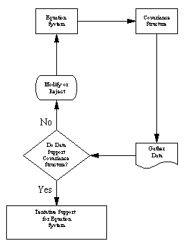
There are some important, and very basic logical points to remember about this process. First, although the mathematical machinery required to perform structural equations modeling is extremely complicated, the basic logic is embodied in the above 5 steps. Below, we diagram the process.

Second, we must remember that it is unreasonable to expect a structural model to fit perfectly — for a number of reasons. A structural model with linear relations is only an approximation. The world is unlikely to be linear. Indeed, the true relations between variables are probably nonlinear. Moreover, many of the statistical assumptions are somewhat questionable as well. The real question is not so much, "Does the model fit perfectly?" but rather, "Does it fit well enough to be a useful approximation to reality, and a reasonable explanation of the trends in our data?"

Third, we must remember that simply because a model fits the data well does not mean that the model is necessarily correct. One cannot prove that a model is true — to assert this is the fallacy of affirming the consequent. For example, we could say "If Joe is a cat, Joe has hair." However, "Joe has hair" does not imply Joe is a cat. Similarly, we can say that "If a certain causal model is true, it will fit the data." However, the model fitting the data does not necessarily imply the model is the correct one. There may be another model that fits the data equally well.

To index

Structural Equation Modeling and the Path Diagram

Path Diagrams play a fundamental role in structural modeling. Path diagrams are like flowcharts. They show variables interconnected with lines that are used to indicate causal flow.

One can think of a path diagram as a device for showing which variables cause changes in other variables. However, path diagrams need not be thought of strictly in this way. They may also be given a narrower, more specific interpretation.

Consider the classic linear regression equation

Y = aX + e

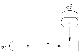
Any such equation may be represented in a path diagram as follows:

Such diagrams establish a simple isomorphism. All variables in the equation system are placed in the diagram, either in boxes or ovals. Each equation is represented on the diagram as follows: All independent variables (the variables on the right side of an equation) have arrows pointing to the dependent variable. The weighting coefficient is placed above the arrow. The above diagram shows a simple linear equation system and its path diagram representation.

Notice that, besides representing the linear equation relationships with arrows, the diagrams also contain some additional aspects. First, the variances of the independent variables, which we must know in order to test the structural relations model, are shown on the diagrams using curved lines without arrowheads attached. We refer to such lines as wires. Second, some variables are represented in ovals, others in rectangular boxes. Manifest variables are placed in boxes in the path diagram. Latent variables are placed in an oval or circle. For example, the variable E in the above diagram can be thought of as a linear regression residual when Y is predicted from X. Such a residual is not observed directly, but calculated from Y and X, so we treat it as a latent variable and place it in an oval.

The example discussed above is an extremely simple one. Generally, we are interested in testing models that are much more complicated than these. As the equation systems we examine become increasingly complicated, so do the covariance structures they imply. Ultimately, the complexity can become so bewildering that we lose sight of some very basic principles. For one thing the train of reasoning which supports testing causal models with linear structural equations testing has several weak links. The variables may be non-linear. They may be linearly related for reasons unrelated to what we commonly view as causality. The ancient adage, "correlation is not causation" remains true, even if the correlation is complex and multivariate. What causal modeling does allow us to do is examine the extent to which data fail to agree with one reasonably viable consequence of a model of causality. If the linear equations system isomorphic to the path diagram does fit the data well, it is encouraging, but hardly proof of the truth of the causal model.

Although path diagrams can be used to represent causal flow in a system of variables, they need not imply such a causal flow. Such diagrams may be viewed as simply an isomorphic representation of a linear equations system. As such, they can convey linear relationships when no causal relations are assumed. Hence, although one might interpret the diagram in the above figure to mean that "X causes Y," the diagram can also be interpreted as a visual representation of the linear regression relationship between X and Y.

To index