Chaoscope Manual

This chapter is an exhaustive description of the attractors found in Chaoscope. The equations are shown here solely for the mathematical inclined (even though some equations may have their validity disputed) as there is no algebra skills involved in rendering attractors. The pictures displayed represent a typical "find" for each equation.

Chaotic Flow, a family of attractors which includes Lorenz and Lorenz-84, is a generalization of the equations described by Pr. Julien Sprott in his paper "Some Simple Chaotic Flows". This is the only equation in Chaoscope where the position of the variables (x, y and z) is itself a parameter, M_i Op. This means that during a Search, not only the parameters are randomized, so is the equation.

This equation was used by Michael Field and Martin Golubitsky to demonstrate how Chaos could yield symmetry.
This attractor is an example of a two dimensional attractor converted to a three dimensional one : values of z are not used for x and y calculations.

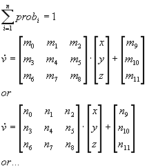
Invented by Michael Barnsley, it is the only attractor with fractal properties available in Chaoscope along with Julia, and probably the most famous of them all. To obtain these convoluted attractors, sets of affine transformations (translation, scale, rotation, etc.) are applied to the orbit in a random order. Each matrix in the equation corresponds to a set of transformation. You can set the number of matrix (from 2 to 8) to use when you create a project or later while a project is already open. Attractors saved under the previous file format (.cla) will have their parameters shown as matrix coefficients instead of affine transformations.

Alan Norton was the first to render Quaternions in the early eighties. He was followed later by John C. Hart, whose code was used for Chaoscope. The inverse of the equation yields a slightly different result than the regular z = z²+ c: the set is perfectly symmetrical. Also, because iterating the equation like a normal attractor proved not very effective, the depth first tracing method has been implemented. The Level parameter defines the depth of the square roots tree. A high level (i.e. > 16) will produce more detail and won't slow down the rendering.

A beautifully simple equation created by Edward Lorenz to demonstrate the chaotic behavior of dynamic systems. This attractor is also historically important because Lorenz discovered, while working on weather patterns simulation, one of the fundamental laws of the Chaos Theory : "the sensitive dependence on initial conditions" he himself dubbed "the butterfly effect".
Although moving the initial orbit won't affect the shape of a strange attractor, the position of the orbit on the attractor after several iterations will vary considerably from one initial position to the other.
Interesting attractors can be found with a relatively high value for dT, i.e. dT > 0.3.

First introduced in Lorenz's paper entitled "Irregularity: a fundamental property of the atmosphere", this equation is a low-dimensional model for long term atmospheric circulation. Rather than a graphical representation of atmospheric currents, the orbit coordinate are the three variables of the model.

Probably the best equation to start experimenting with, since the orbit will never escape the attractor as it is "trapped" in sinusoids. A good set of parameters is {1, 1.8, 0.71, 1.51} from which nice attractors can be found, after modifying each parameter slightly.

The Polynomial type A (which probably is polynomial only by name !) uses the most simple equation, it is therefore the fastest attractor to render. The equation is a special case of Type B where P1, P3 and P5 = 0.

A slightly more complex equation for a challenging specimen. This attractor equation is rather feeble and will see the orbit escapes more than often. When not escaping, it won't produce a great variety of shapes.

Next step up the Polynomial evolution ladder, it has three times more parameters than its predecessor. This equation is a good compromise between speed and complexity.

Polynomial Function is a group of three equations which make use of algebraic or trigonometric functions rather than the normal 2^nd order structure. They were adapted to 3 dimensions from Julien Sprott's book on Strange Attractors. Abs will yield very typical angular forms, Power will add some flexibility to Abs straight lines, while Sin will produce wavy attractors.

Described in Pr. Julien Sprott's book under its scientific name, "three dimensional quadratic map", it is the most complex equation found in Chaoscope.
Given the number of parameters, and if you were to limit your choice to 20 values for each of them, it allows 20³⁰ combinations, which means you would have virtually one chance out of 1,073,741,824,000,000,000,000,000,000,000,000,000,000 to reproduce a strange attractor without knowing its original parameters. It would be like searching for a needle in a thirty dimensional stack of hay. You can set the order of the equation (from the 2^nd to the 5^th) when you create a project or later while a project is already open.

The only equation created for Chaoscope. The idea was to have an attractor from which the orbit couldn't escape, regardless of its parameters, without using trigonometric functions (like Pickover does) thus achieving a relatively good rendering speed.
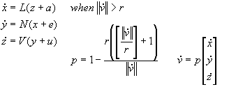
The first attempt was to use a polynomial-like equation, and limit the volume the orbit could evolve into to a unit cube. Each time the orbit was leaving the cube space it would reappear near the opposite face, inside the cube. The best result obtained was remotely looking like a Menger Sponge. Later, the cube was replaced by a sphere of radius R and the equation was simplified. The best looking attractors are found setting R to a negative value, which makes no sense considering the concept behind the equation, leaving the author puzzled.