The Chaos Hypertextbook™
© 1995-2003 by Glenn Elert
All Rights Reserved -- Fair Use Encouraged
Julia sets rendered with Object Mandelbrot & Julia's Dream
Let's return for a while to our original map
f: x --> x2 + c.
The graph of this function is a parabola when "x" and "c" are real numbers. The orbits of well-behaved seeds are bounded for parameter values in the interval [-2, 1/4]. These orbits can settle on to attracting fixed points, be periodic, or ergodic. A small set of fixed points, the repelling fixed points, do not generate orbits in the traditional sense. They neither roam nor run off to infinity and one need not wait for them to exhibit "characteristic" behavior. They are permanently and immutably fixed and nearby points avoid them. They lie on the frontier between those seeds with bounded orbits and those with unbounded orbits. Such is the behavior in general for all points and all parameter values; or is it? The discussion so far has been constrained by a prejudice for real numbers. What happens when we admit that i = sqrt(-1) has a solution? How does our function behave when "z" and "c" are complex numbers? The answer, of course, is the same but the results are much more interesting than such a flip statement implies.
The map
f: z --> z2 + c
is equivalent to the two-dimensional map
f: (x, y) --> (x2 - y2 + a, 2xy + b)
where z = x + iy = (x, y) is a point to be iterated and c = a + ib = (a, b) acts as the parameter. Thus, the quadratic map of the complex numbers can be studied as a family of transformations to the complex plane.
|
|
|
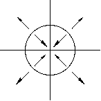
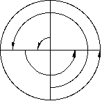
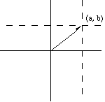
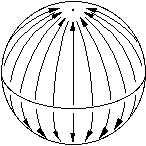
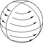
| Stretch points inside the unit circle towards the origin. Stretch points outside towards infinity. | Wrap the plane around itself once without cutting or tearing such that every every angle value has doubled. | Shift the plane over so the origin lies on (a, b). |
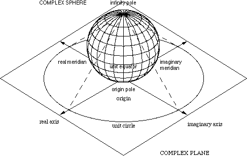
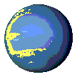
Actually, it's easier to discuss these transformations if we represent the complex numbers as points on a complex sphere. The origin would be one pole and infinity another pole with the unit sphere being the equator. Imagine placing a light bulb at the infinity pole. Points on the sphere would leave shadows in unique positions on the plane. The complex plane is thus a projection of the complex sphere. While this is easier to deal with because we have a single point called infinity, it is not easier to diagram. Let's give it a shot.
Stereographic Projection of the Complex Sphere on to the Complex
Plane
 |
 |
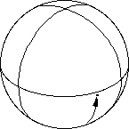 |
| Stretch points below the unit equator towards the origin pole. Stretch points above the equator towards the infinity pole. | Wrap the sphere around itself once without cutting or tearing such that every longitude value has doubled. | Stretch the sphere so the origin pole shifts to the point (a, b) but the infinity pole stays fixed. |
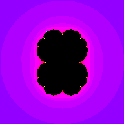
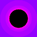
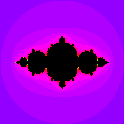
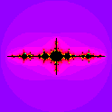
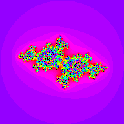
This family of mappings is said to be conformal; that is, it leaves angles unchanged. Despite all this stretching, twisting, and shifting there is always a set of points that transforms into itself. Such sets are called the Julia sets after the French mathematician Gaston Julia who first conceived of them in the 1910s. The special case of c = (0, 0) has already been dealt with (the set is the unit circle). Let's look at a variety of parameter values and see what kind of Julia sets arise. Some examples are shown below.
 |
 |
 |
 |
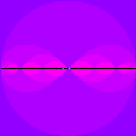
| c = 0.275 | c = 1/4 | c = 0 | c = -3/4 |
 |
 |
 |
 |
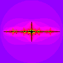
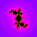
| c = -1.312 | c = -1.375 | c = -2 | c = i |
 |
 |
 |
 |
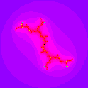
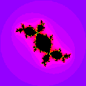
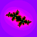
| c = (+0.285, +0.535) | c = (-0.125, +0.750) | c = (-0.500, +0.563) | c = (-0.687, +0.312) |
Sets on the real axis are reflection symmetric while those with complex parameter values show rotational symmetry. With the exception of the parameter value c = 0, all Julia sets exhibit self-similarity. There are two broad categories of Julia sets: those which are connected and those which are not. Of the twelve examples shown, only the first and last are disconnected. The distinction between the two categories is extreme. Disconnected sets are completely disconnected into a countably infinite assembly of isolated points. In addition, these points are arranged in dense groups such that any finite disk surrounding a point contains at least one other point in the set. Such sets are said to be dustlike. As they can be shown to be similar to the Cantor middle thirds set, they are often called Cantor dusts. In contrast, the connected sets are completely connected. Topologically, they are either equivalent to a severely deformed circle or to a line with an infinite series of branches and sub-branches called a dendrite (at c = i for example).
| Another quality webpage by Glenn Elert |
 |
home | contact bent | chaos | eworld | facts | physics |