Virtual Laboratories > Finite Sampling Models > 1 2 3 4 [5] 6 7 8 9 10
Suppose that the objects in our population are numbered from 1 to N, so that D = {1, 2, ..., N}. For example, the population might consist of manufactured items, and the labels might correspond to serial numbers. We sample n objects at random, without replacement from D:
X = (X1, X2, ..., Xn), where Xi in D is the i'th object chosen.
Recall that X is uniformly distributed over the set of permutations of size n chosen from D. Recall also that W = {X1, X2, ..., Xn} is the unordered sample, which is uniformly distributed on the set of combinations of size n chosen from D.
For i = 1, 2, ..., n, let X(i) denote the i'th smallest of X1, X2, ..., Xn. The random variable X(i) is known as the i'th order statistic of the sample. Note that in particular, X(1) is the minimum score and X(n) is the maximum score.
![]() 1. Show that X(i)
takes values i, i + 1, ..., N - n + i.
1. Show that X(i)
takes values i, i + 1, ..., N - n + i.
We will denote the vector of order statistics by
U = (X(1), X(2), ..., X(n)).
Note that U takes values in L = {(x1,
x2, ..., xn): 1 ![]() x1 < x2 < ··· < xn
x1 < x2 < ··· < xn
![]() N}
N}
![]() 2. Run the
order statistic
experiment. Note that you can vary the population size N
and the sample size n. The order statistics are recorded on each update.
2. Run the
order statistic
experiment. Note that you can vary the population size N
and the sample size n. The order statistics are recorded on each update.
![]() 3. Show
that L has C(N, n) elements and that U
is uniformly distributed on L.
3. Show
that L has C(N, n) elements and that U
is uniformly distributed on L.
Hint: U = (x1, x2,
..., xn) if and only if W = {x1,
x2, ..., xn} if and only if X
is one of the n! permutations of (x1, x2,
..., xn).
![]() 4. Use a
combinatorial argument to show that the density
function of X(i) is as follows:
4. Use a
combinatorial argument to show that the density
function of X(i) is as follows:
P(X(i) = k) = C(k - 1, i - 1)C(N - k, n - i) / C(N, n) for k = i, i + 1, ..., N - n + i.
![]() 5. In the
order statistic
experiment, vary the parameters and note the shape of
the density function. Now with N = 30, n = 10 and i = 5, run
the experiment 1000 times, updating very 10 runs. Note the apparent convergence of the
empirical density function to the true density function.
5. In the
order statistic
experiment, vary the parameters and note the shape of
the density function. Now with N = 30, n = 10 and i = 5, run
the experiment 1000 times, updating very 10 runs. Note the apparent convergence of the
empirical density function to the true density function.
The density function in Exercise 4 can be used to obtain an interesting identity involving the binomial coefficients. This identity, in turn, can be used to find the mean and variance of X(i) .
![]() 5.
Show that for each i = 1, 2,
..., N,
5.
Show that for each i = 1, 2,
..., N,
![]() k
= i, ..., N - n + i C(k, i)
C(N - k, n - i) = C(N + 1, n
+ 1).
k
= i, ..., N - n + i C(k, i)
C(N - k, n - i) = C(N + 1, n
+ 1).
![]() 6. Use the
identity in the Exercise 5 to show that
6. Use the
identity in the Exercise 5 to show that
E(X(i)) = i (N + 1) / (n + 1).
![]() 7. Use the
identity in Exercise 5 to show that
7. Use the
identity in Exercise 5 to show that
var(X(i)) = (N + 1)(N - n)i(n + 1 - i) / [(n + 1)2(n + 2)].
![]() 8. In
the order statistic
experiment, vary the parameters and note the size
and location of the mean/standard deviation bar. Now with N = 30, n = 10
and i = 5, run the experiment 1000 times, updating very 10 runs. Note the
apparent convergence of the empirical moments to the true moments.
8. In
the order statistic
experiment, vary the parameters and note the size
and location of the mean/standard deviation bar. Now with N = 30, n = 10
and i = 5, run the experiment 1000 times, updating very 10 runs. Note the
apparent convergence of the empirical moments to the true moments.
![]() 10. Suppose that
in a lottery, tickets numbered from 1 to 25 are placed in a bowl. Five tickets are chosen
at random and without replacement. Compute
10. Suppose that
in a lottery, tickets numbered from 1 to 25 are placed in a bowl. Five tickets are chosen
at random and without replacement. Compute
![]() 11. Use the
result of Exercise 6 to show that for i = 1, 2, ..., n, the following
statistic is an unbiased estimator of N:
11. Use the
result of Exercise 6 to show that for i = 1, 2, ..., n, the following
statistic is an unbiased estimator of N:
Wi = [(n + 1) X(i) / i] - 1.
Since Wi is unbiased, its variance is the mean square error, a measure of the quality of the estimator.
![]() 12. Show that var(Wi)
= (N + 1)(N - n)(n + 1 - i) / [i(n
+ 2)]
12. Show that var(Wi)
= (N + 1)(N - n)(n + 1 - i) / [i(n
+ 2)]
![]() 13. Show that for
fixed N and n, var(Wi) decreases as i
increases.
13. Show that for
fixed N and n, var(Wi) decreases as i
increases.
Thus, the estimators improve as i increases; in particular, Wn is the best and W1 the worst.
![]() 14. Show that var(Wj)
/ var(Wi) = j(n + 1 - i) / [i(n
+ 1 - j)]
14. Show that var(Wj)
/ var(Wi) = j(n + 1 - i) / [i(n
+ 1 - j)]
This ratio is known as the relative efficiency of Wi with respect to Wj.
Usually, we hope that an estimator improves (in the sense of mean square error) as the sample size n increases (the more information we have, the better our estimate should be). This general idea is known as consistency.
![]() 15. Show that the
var(Wn) decreases to 0 as n increases to N.
15. Show that the
var(Wn) decreases to 0 as n increases to N.
![]() 16. Show that for
fixed i, var(Wi) at first increases and then decreases to 0
as n increases from 1 to N.
16. Show that for
fixed i, var(Wi) at first increases and then decreases to 0
as n increases from 1 to N.
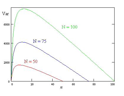
The following graph, due to Christine Nickel, shows var(W1) as a function of n for N = 50, 75, and 100.
The estimator Wn was used by the Allies during World War II to estimate the number of German tanks N that had been produced. German tanks had serial numbers, and captured German tanks and captured records formed the sample data. According to Richard Larsen and Morris Marx, this estimate of German tank production in 1942 was 3400, very close the the true number.
![]() 17. Suppose that
in a certain war, 100 enemy tanks have been captured. The largest serial number of the
captured tanks is 1423. Estimate the total number of tanks that have been produced.
17. Suppose that
in a certain war, 100 enemy tanks have been captured. The largest serial number of the
captured tanks is 1423. Estimate the total number of tanks that have been produced.
![]() 18. In
the order statistic
experiment, and set N = 100 and n =
10. Run the experiment 50 times, updating after each run. For each run, compute the
estimate of N based on each order statistic. For each estimator, compute the square
root of the average of the squares of the errors over the 50 runs. Based on these
empirical error estimates, rank the estimators of N in terms of quality.
18. In
the order statistic
experiment, and set N = 100 and n =
10. Run the experiment 50 times, updating after each run. For each run, compute the
estimate of N based on each order statistic. For each estimator, compute the square
root of the average of the squares of the errors over the 50 runs. Based on these
empirical error estimates, rank the estimators of N in terms of quality.
![]() 19. Suppose that
in a certain war, 100 enemy tanks have been captured. The smallest serial number of the
captured tanks is 23. Estimate the total number of tanks that have been produced.
19. Suppose that
in a certain war, 100 enemy tanks have been captured. The smallest serial number of the
captured tanks is 23. Estimate the total number of tanks that have been produced.
If the sampling is with replacement, then the sample variables X1, X2, ..., Xn are independent and identically distributed. The order statistics from such samples are studied in the chapter on Random Samples.