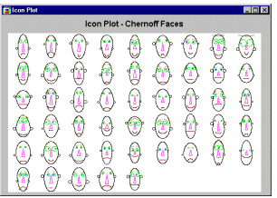
Icon Plots - Chernoff Faces. Chernoff faces is the most "elaborate" type of icon plot. A separate "face" icon is drawn for each case; relative values of the selected variables for each case are assigned to shapes and sizes of individual facial features (e.g., length of nose, angle of eyebrows, width of face).

See also Graphical Analytic Techniques: Icon Plots.

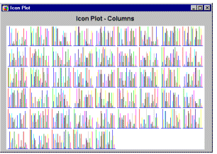
Icon Plots - Columns. In this type of icon plot, an individual column graph is plotted for each case; relative values of the selected variables for each case are represented by the height of consecutive columns.

See also Graphical Analytic Techniques: Icon Plots.

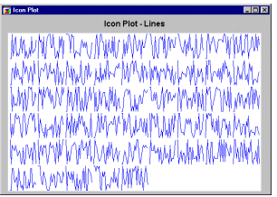
Icon Plots - Lines. In this type of icon plot, an individual line graph is plotted for each case; relative values of the selected variables for each case are represented by the height of consecutive break points of the line above the baseline.

See also Graphical Analytic Techniques: Icon Plots.

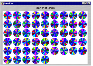
Icon Plots - Pies. In this type of icon plot, data values for each case are plotted as a pie chart (clockwise, starting at 12:00); relative values of selected variables are represented by the size of the pie slices.

See also Graphical Analytic Techniques: Icon Plots.

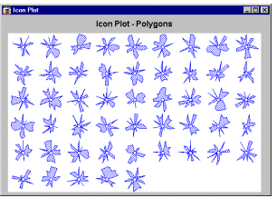
Icon Plots - Polygons. In this type of icon plot, a separate polygon icon is plotted for each case; relative values of the selected variables for each case are represented by the distance from the center of the icon to consecutive corners of the polygon (clockwise, starting at 12:00).

See also Graphical Analytic Techniques: Icon Plots.

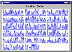
Icon Plots - Profiles. In this type of icon plot, an individual area graph is plotted for each case; relative values of the selected variables for each case are represented by the height of consecutive peaks of the profile above the baseline.

See also Graphical Analytic Techniques: Icon Plots.

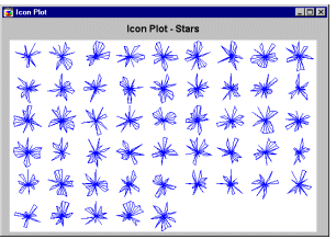
Icon Plots - Stars. In this type of icon plot, a separate star-like icon is plotted for each case; relative values of the selected variables for each case are represented (clockwise, starting at 12:00) by the relative length of individual rays in each star. The ends of the rays are connected by a line.

See also Graphical Analytic Techniques: Icon Plots.

Icon Plots - Sun Rays. In this type of icon plot, a separate sun-like icon is plotted for each case; each ray represents one of the selected variables (clockwise, starting at 12:00), and the length of the ray represents 4 standard deviations. Data values of the variables for each case are connected by a line.

See also Graphical Analytic Techniques: Icon Plots.

Incremental (vs. Non-Incremental Learning Algorithms). Methods (algorithms) for predictive data mining are also referred to as "learning" algorithms, because they derive information from the data to predict new observations. These algorithms can be divided into those that require one or perhaps two complete passes through the input data, and those that require iterative multiple access to the data to complete the estimation. The former type of algorithms are also sometimes referred to as incremental learning algorithms, because they will complete the computations necessary to fit the respective models by processing one case at a time, each time "refining" the solution; then, when all cases have been processed, only few additional computations are necessary to produce the final results. Non-incremental learning algorithms are those that need to process all observations in each iteration of an iterative procedure for refining a final solution. Obviously, incremental learning algorithms are usually much faster than non-incremental algorithms, and for extremely large data sets, non-incremental algorithms may not be applicable at all (without first sub-sampling).

Independent Events. Two events are independent if the occurrence of one of the events gives us no information about whether or not the other event will occur; that is, the events have no influence on each other.

Independent vs. Dependent Variables. The terms dependent and independent variable apply mostly to experimental research where some variables are manipulated, and in this sense they are "independent" from the initial reaction patterns, features, intentions, etc. of the subjects. Some other variables are expected to be "dependent" on the manipulation or experimental conditions. That is to say, they depend on "what the subject will do" in response. Independent variables are those that are manipulated whereas dependent variables are only measured or registered.

Somewhat contrary to the nature of this distinction, these terms are also used in studies where we do not literally manipulate independent variables, but only assign subjects to "experimental groups" based on some preexisting properties of the subjects. For example, if in an experiment, males are compared with females regarding their white cell count (WCC), Gender could be called the independent variable and WCC the dependent variable.

See Dependent vs. independent variables for more information.

Inertia. The term inertia in correspondence analysis is used by analogy with the definition in applied mathematics of "moment of inertia," which stands for the integral of mass times the squared distance to the centroid (e.g., Greenacre, 1984, p. 35). Inertia is defined as the total Pearson Chi-square for a two-way frequency table divided by the total sum of all observations in the table.

In-Place Database Processing (IDP). In-Place Database Processing (IDP) is an advanced database access technology developed at StatSoft to support high-performance, direct interface between external data sets residing on remote servers and the analytic functionality of data analysis software (such as STATISTICA products) residing on the client computers. The IDP technology has been developed to facilitate accessing data in large databases using a one-step process which does not necessitate creating local copies of the data set. IDP significantly increases the overall performance of data processing software; it is particularly well suited for large data mining and exploratory data analysis tasks.

The source of the IDP performance gains. The speed gains of the IDP technology - over accessing data in a traditional way - result not only from the fact that IDP allows the client data analysis software to access data directly in databases and skip the otherwise necessary step of first importing the data and creating a local data file, but also from its "multitasking" (technically, asynchronous and distributed processing) architecture. Specifically, IDP uses the processing resources (multiple CPUs) of the database server computers to execute the query operations, extract the requested records of data and send them to the client computer, while the data analysis software on the client computer is simultaneously processing these records as they arrive.

Interactions. An effect of interaction occurs when a relation between (at least) two variables is modified by (at least one) other variable. In other words, the strength or the sign (direction) of a relation between (at least) two variables is different depending on the value (level) of some other variable(s). (The term interaction was first used by Fisher, 1926). Note that the term "modified" in this context does not imply causality but represents a simple fact that depending on what subset of observations (regarding the "modifier" variable(s)) you are looking at, the relation between the other variables will be different.

For example, imagine that we have a sample of highly achievement-oriented students and another of achievement "avoiders." We now create two random halves in each sample, and give one half of each sample a challenging test, the other an easy test. We measure how hard the students work on the test. The means of this (fictitious) study are as follows:

	Achievement- oriented	Achievement- avoiders
Challenging Test Easy Test	10   5	5 10

How can we summarize these results? Is it appropriate to conclude that (1) challenging tests make students work harder, (2) achievement-oriented students work harder than achievement-avoiders? None of these statements captures the essence of this clearly systematic pattern of means. The appropriate way to summarize the result would be to say that challenging tests make only achievement-oriented students work harder, while easy tests make only achievement-avoiders work harder. In other words, the relation between the type of test and effort is positive in one group but negative in the other group. Thus, the type of achievement orientation and test difficulty interact in their effect on effort; specifically, this is an example of a two-way interaction between achievement orientation and test difficulty. (Note that statements 1 and 2 above would describe so-called main effects.)

For more information regarding interactions, see Interaction Effects in the ANOVA chapter.

Interpolation. Projecting a curve between known data points to infer the value of a function at points between.

Interval Scale. This scale of measurement allows you to not only rank order the items that are measured, but also to quantify and compare the sizes of differences between them (no absolute zero is required).

See also, Measurement scales.

Intraclass Correlation Coefficient. The value of the population intraclass correlation coefficient is a measure of the homogeneity of observations within the classes of a random factor relative to the variability of such observations between classes. It will be zero only when the estimated effect of the random factor is zero and will reach unity only when the estimated effect of error is zero, given that the the total variation of the observations is greater than zero (see Hays, 1988, p. 485).

Note that the population intraclass correlation can be estimated using variance component estimation methods. For more information see the chapter on Variance Components and Mixed-Model ANOVA/ANCOVA.

Invariance Under a Constant Scale Factor (ICSF). A structural model is invariant under a constant scale factor (ICSF) if model fit is not changed if all variables are multiplied by the same constant. Most, but not all, structural models that are of practical interest are ICSF (see Structural Equation Modeling).

Invariance Under Change of Scale (ICS). A structural model is invariant under change of scale if model fit is not changed by rescaling the variables, i.e., by multiplying them by scale factors (see Structural Equation Modeling).

Inverse Document Frequency. The inverse document frequency is a useful transformation of raw word frequency counts computed in the context of text mining, in order to simultaneously express the frequencies with which specific terms or words are used in a collection of documents, as well as their semantic specificities, i.e., the extent to which particular words are used only in specific documents in the collection.

Suppose you index a collection of text documents and compute the word frequencies (wf) to enumerate the number of times that each word or term is used in each document. A particular issue that you may want to consider more carefully, and reflect in the indices used in further analyses, are the relative document frequencies (df) of different words. For example, a term such as "guess" may occur frequently in all documents, while another term such as "software" may only occur in a few. The reason is that one might make "guesses" in various contexts, regardless of the specific topic, while "software" is a more semantically focused term that is likely to occur only in documents that deal with computer software. A common and very useful transformation that reflects both the semantic specificity of words (document frequencies) as well as the overall frequencies of their occurrences (word frequencies) is the so-called inverse document frequency (for word i and document j):

In this formula (see also formula 15.5 in Manning and Schütze, 2002), N is the total number of documents, and dfi is the document frequency for the i'th word (the number of documents that include this word). Hence, it can be seen that this formula includes both a dampening of the simple word frequencies via a log function, and also includes a weighting factor that evaluates to 0 if the word occurs in all documents (log(N/N=1)=0), and to the maximum value when a word only occurs in a single document (log(N/1)=log(N)). It can easily be seen how this transformation will create indices that both reflect the relative frequencies-of-occurrences of words, as well as their semantic specificities over the documents included in the analysis. For more information, see Manning and Schütze (2002).

Ishikawa Chart. A type of diagram used to depict the factors or variables that make up a process; named after Professor Kaoru Ishikawa of Tokyo University (e.g., see Seder, 1962), this diagram is also referred to as the Cause-and-Effect diagram.

For details, see Cause-and-Effect Diagram; see also Cause-and-Effect Diagrams in the Introductory Overview of Process Analysis.

Isotropic Deviation Assignment. An algorithm for assigning radial unit deviations, which selects a single deviation value using a heuristic calculation based on the number of units and the volume of pattern space they occupy, with the objective of ensuring "a reasonable overlap." (Haykin, 1994).

See also the Neural Networks chapter.

IV. IV stands for Independent Variable. See also Independent vs. Dependent Variables.

JPEG. Acronym for Joint Photographic Experts Group. An ISO/ITU standard for storing images in compressed form using a discrete cosine transform.

Jacobian Matrix. The first-order derivative of a continuous and differentiable function F (of multiple parameters) is sometimes called the Jacobian matrix J of F (at some specific values of parameter vector x). The Jacobian matrix plays an important role in most computational algorithms for estimating parameter values for nonlinear regression problems, in particular in the Gauss-Newton and Levenberg-Marquardt algorithms; see also Nonlinear Estimation for details.

Jogging Weights. Adding a small random amount to the weights in a neural network, in an attempt to escape a local optima in error space.

See also the Neural Networks chapter.

Johnson Curves. Johnson (1949) described a system of frequency curves that represents transformations of the standard normal curve (see Hahn and Shapiro, 1967, for details). By applying these transformations to a standard normal variable, a wide variety of non-normal distributions can be approximated, including distributions which are bounded on either one or both sides (e.g., U- shaped distributions). The advantage of this approach is that once a particular Johnson curve has been fit, the normal integral can be used to compute the expected percentage points under the respective curve. Methods for fitting Johnson curves, so as to approximate the first four moments of an empirical distribution, are described in detail in Hahn and Shapiro, 1967, pages 199-220; and Hill, Hill, and Holder, 1976.

See also, Pearson Curves.

Join. A join shows how data is related between two tables. When two tables contain matching values on a field, records from the two tables can be combined by defining a Join. For example, suppose one table has the weight of objects with their associated part number and another table has part numbers and their associated product names. A join specifies that the two part number fields are equivalent and allows weights and product names to be related.

Joining Networks (in Neural Networks). It is sometimes useful to be able to join two networks together to form a single composite network for a number of reasons:

• You might train one network to do preprocessing of data, and another to further classify the preprocessed data. Once completed, the networks can be joined together to classify raw data.

• You might want to add a loss matrix to a classification network, to make minimum cost decisions.

Note: Networks can only be joined if the number of input neurons in the second network matches the number of output neurons in the first network. The input neurons from the second network are discarded, and their fan-out weights are attached to the output neurons of the first network.

Caution: The post-processing information from the first network and the input preprocessing information from the second network are also discarded. The composite network is unlikely to make sense unless you have designed the two networks with this in mind; i.e., with no post-processing performed by the first network and no preprocessing performed by the second network.

Kendall Tau. Kendall tau is equivalent to the Spearman R statistic with regard to the underlying assumptions. It is also comparable in terms of its statistical power. However, Spearman R and Kendall tau are usually not identical in magnitude because their underlying logic, as well as their computational formulas are very different. Siegel and Castellan (1988) express the relationship of the two measures in terms of the inequality:

-1 < = 3 * Kendall tau - 2 * Spearman R < = 1

More importantly, Kendall tau and Spearman R imply different interpretations: While Spearman R can be thought of as the regular Pearson product-moment correlation coefficient as computed from ranks, Kendall tau rather represents a probability. Specifically, it is the difference between the probability that the observed data are in the same order for the two variables versus the probability that the observed data are in different orders for the two variables. Kendall (1948, 1975), Everitt (1977), and Siegel and Castellan (1988) discuss Kendall tau in greater detail. Two different variants of tau are computed, usually called tau_b and tau_c. These measures differ only with regard as to how tied ranks are handled. In most cases these values will be fairly similar, and when discrepancies occur, it is probably always safest to interpret the lowest value.

Kernel functions. Simple functions (typically Gaussians) which are added together, positioned at known data points, to approximate a sampled distribution (Parzen, 1962).

See also the Neural Networks chapter.

K-Means algorithm (in Neural Networks). The K-means algorithm (Moody and Darkin, 1989; Bishop, 1995) assigns radial centers to the first hidden layer in the network if it consists of radial units.

K-means assigns each training case to one of K clusters (where K is the number of radial units), such that each cluster is represented by the centroid of its cases, and each case is nearer to the centroid of its cluster than to the centroids of any other cluster. It is the centroids that are copied to the radial units.

The intention is to discover a set of cluster centers which best represent the natural distribution of the training cases.

Technical Details. K-means is an iterative algorithm. The clusters are first formed arbitrarily by choosing the first K cases, assigning each subsequent case to the nearest of the K, then calculating the centroids of each cluster.

Subsequently, each case is tested to see whether the center of another cluster is closer than the center of its own cluster; if so, the case is reassigned. If cases are reassigned, the centroids are recalculated and the algorithm repeats.

Caution. There is no formal proof of convergence for this algorithm, although in practice it usually converges reasonably quickly.

See also, the Neural Networks chapter.

Kohonen Algorithm (in Neural Networks). The Kohonen algorithm (Kohonen, 1982; Patterson, 1996; Fausett, 1994) assigns centers to a radial hidden layer by attempting to recognize clusters within the training cases. Cluster centers close to one another in pattern-space tend to be assigned to units that are close to each other in the network (topologically ordered).

The Kohonen training algorithm is the algorithm of choice for Self Organizing Feature Map networks. It can also be used to train the radial layer in other network types; specifically, radial basis function, cluster, and generalized regression neural networks.

SOFM networks are typically arranged with the radial layer laid out in two dimensions. From an initially random set of centers, the algorithm tests each training case and selects the nearest center. This center and its neighbors are then updated to be more like the training case.

Over the course of the algorithm, the learning rate (which controls the degree of adaptation of the centers to the training cases) and the size of the neighborhood are gradually reduced.  In the early phases, therefore, the algorithm assigns a rough topological map, with similar clusters of cases located in certain areas of the radial layer. In later phases the topological map is fine-tuned, with individual units responding to small clusters of similar cases.

If the neighborhood is set to zero throughout, the algorithm is a simple cluster-assignment technique. It can also be used on a one-dimensional layer with or without neighborhood definition.

If class labels are available for the training cases, then after Kohonen training, labels can be assigned using class labeling algorithms and Learned Vector Quantization used to improve the positions of the radial exemplars.

Technical Details. The Kohonen update rule is:

x is the training case,

h(t) is the learning rate.

Kohonen Training. An algorithm which assigns cluster centers to a radial layer by iteratively submitting training patterns to the network, and adjusting the winning (nearest) radial unit center, and its neighbors, towards the training pattern (Kohonen, 1982; Fausett, 1994; Haykin, 1994; Patterson, 1996).

See also, the Neural Networks chapter.

Kolmogorov-Smirnov test. The Kolmogorov-Smirnov one-sample test for normality is based on the maximum difference between the sample cumulative distribution and the hypothesized cumulative distribution. If the D statistic is significant, then the hypothesis that the respective distribution is normal should be rejected. For many software programs, the probability values that are reported are based on those tabulated by Massey (1951); those probability values are valid when the mean and standard deviation of the normal distribution are known a-priori and not estimated from the data. However, usually those parameters are computed from the actual data. In that case, the test for normality involves a complex conditional hypothesis ("how likely is it to obtain a D statistic of this magnitude or greater, contingent upon the mean and standard deviation computed from the data"), and the Lilliefors probabilities should be interpreted (Lilliefors, 1967). Note that in recent years, the Shapiro-Wilks' W test has become the preferred test of normality because of its good power properties as compared to a wide range of alternative tests.

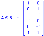
Kronecker Product. The Kronecker (direct) product of 2 matrices A, with p rows and q columns, and B, with m rows and n columns, is the matrix with pm rows and qn columns given by

A Ä B = a _ij B

For example, if

and

then

Kronecker Product matrices have a number of useful properties (for a summary of these properties, see Hocking, 1985).

Kruskall-Wallis test. The Kruskall-Wallis test is a non-parametric alternative to one-way (between-groups) ANOVA. It is used to compare three or more samples, and it tests the null hypothesis that the different samples in the comparison were drawn from the same distribution or from distributions with the same median. Thus, the interpretation of the Kruskall-Wallis test is basically similar to that of the parametric one-way ANOVA, except that it is based on ranks rather than means. For more details, see Siegel & Castellan, 1988. See also, Nonparametric Statistics.

Kurtosis. Kurtosis (the term first used by Pearson, 1905) measures the "peakedness" of a distribution. If the kurtosis is clearly different than 0, then the distribution is either flatter or more peaked than normal; the kurtosis of the normal distribution is 0. Kurtosis is computed as:

Kurtosis = [n*(n+1)*M₄ - 3*M₂*M₂*(n-1)]/[(n-1)*(n-2)*(n-3)*⁴]

where:
M_j     is equal to: (x_i-Mean_x)^j
 n       is the valid number of cases
⁴     is the standard deviation (sigma) raised to the fourth power

See also, Descriptive Statistics.